Understanding how perspective projection and camera positioning work together in order to create realistic views of 3d objects.
Today we'll continue our foray into the 3D viewing pipeline of computer graphics. Last time,
we touched on some WebGL fundamentals and discussed oblique projection as a way to view three dimensional things on two dimensional screens.
Oblique projection is mainly used in technical drawings, as it does a relatively good job at conveying the three-dimensional shape of an object
in two dimensions while remaining easy to draw. However, views obtained from this type of projection do not appear fully realistic. Perspective projection
does a better job at conveying realistic views of three-dimensional images, because it more closely resembles how light hits our eyes in reality.
Combined with a camera abstraction, computer graphics is able to fool your eye into seeing a rotating bunny in the animation above, even though what we're actually
doing is staring at a 2-dimensional array of pixels.
In this article, we will discuss the math behind perspective projection and the camera abstraction, including the peculiarities required to make
this work in WebGL. Reading
the previous article on oblique projection.
is not required, but might be interesting anyway.
Perspective Projection of Vertices.
A 3d model, like the one of the bunny above, consists of an list of vertices and their (x,y,z) coordinates, and a list of faces, each
face specifying the vertices that define it. Commonly in computer graphics, triangles are the primitive of choice for faces. Thus, each face is specified by
listing three vertices that define the edges of the triangle.
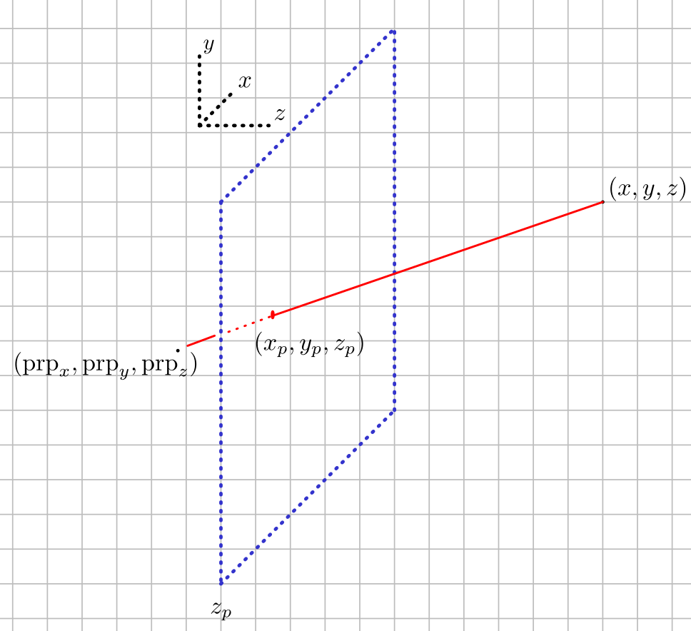
We can obtain a perspective projection of a 3d model by specifying a projection reference point and a projection plane. Then, we take each of the
vertices making up the 3d model and project the coordinates onto the plane along the line connecting the coordinate and the projection reference point.
The following sketch illustrates the situation.
To be clear, what we want to calculate for the perspective projection is \(x_p\) and \(y_p\). The projection reference point and the offset
\(z_p\) of the projection plane is something we specify [1], and the coordinate \(x,y,z\) belongs to the 3d model we would like to project onto the plane.
To get \(x_p\) and \(y_p\), we acknowledge that both points lie somewhere on the line connecting \((\text{prp}_x, \text{prp}_y, \text{prp}_z)\)
and \((x,y,z)\). In other words, for some \(u\) with \(0 \leq u \leq 1\):
$$
\begin{align}
x_p &= x + u (\text{prp}_x - x), \\
y_p &= y + u (\text{prp}_y - y), \\
z_p &= z + u (\text{prp}_z - z).\\
\end{align}
$$
Noting again that we know \(z_p\), we can solve this equation for \(u\):
$$
u = \dfrac{z_p-z}{\text{prp}_z - z},
$$
and plug the result into the equations for \(x_p\) and \(y_p\):
$$
\begin{align}
x_p &= \text{prp}_x + \dfrac{z_p-z}{\text{prp}_z - z}(\text{prp}_x - x), \\
y_p &= \text{prp}_y + \dfrac{z_p-z}{\text{prp}_z - z}(\text{prp}_y - y). \\
\end{align}
$$
This is really all there is to the math, but in order to compute the perspective projection efficiently we would like
to represent this calculation as a matrix-vector multiplication in homogeneous coordinates of the form
$$
\begin{bmatrix}x_h\\y_h\\z_h\\h\end{bmatrix}=P \begin{bmatrix}x\\y\\z\\1\end{bmatrix}.
$$
This has been discussed in more detail in the
article about orthographic perspective, but the gist is that the final computation result is
determined by dividing through \(h\), for example
$$
x_p = \dfrac{x_h}{h},
$$
and the sole reason this is done is that this approach is flexible enough to represent all common computer graphics projections and
as a result, hardware is optimized for it.
Thankfully, looking at the equations for \(x_p\) and \(y_p\) above we see that they are easily rearranged to conform to this scheme: from
$$
x_p = \dfrac{1}{\text{prp}_z - z} (x\ (\text{prp}_z - z_p) - z\ \text{prp}_x + z_p \text{prp}_x)
$$
we see that \(h\) must be \(\text{prp}_z - z\), and \(x_h\) must be the remaining term in parentheses. With \(y_p\) computed analogously, we
can express this computation as the desired matrix-vector multiplication
$$
\begin{bmatrix}x_h\\y_h\\z_h\\h\end{bmatrix}= P \boldsymbol{x} =
\begin{bmatrix}
\text{prp}_z-z_p & 0 & -\text{prp}_x & z_p\ \text{prp}_x \\
0 & \text{prp}_z-z_p & -\text{prp}_y & z_p\ \text{prp}_y \\
0 & 0 & 1 & 0 \\
0 & 0 & -1 & \text{prp}_z\\
\end{bmatrix}
\begin{bmatrix}x\\y\\z\\1\end{bmatrix}.
$$
The variables appearing in this projection matrix are what you can manipulate in the title animation of the bunny.
Note that varying \(\text{prp}_x\) and \(\text{prp}_y\) is slightly uninteresting, only slightly changing the angle of projection. It is not
a surprise that often times, the \(\text{prp}\) vector is placed on the origin, which of course also drastically simplifies the matrix above.
Something more interesting happens when varying \(z_p\) in relation to \(\text{prp}_z\): If \(\text{prp}_z < z_p\), the image flips upside down!
The reason this happens becomes apparent when looking at the sketch again: the reference point of projection is now between the projection
plane and the object [2].
Camera Positioning.
Next to the perspective projection, the other important aspect of generating realistic 3-dimensional views of objects is the ability
to view them from arbitrary angles. The abstraction that is used in computer graphics is that of a camera pointing at the object.
In the case of WebGL, recall that in the end, the library draws anything that is inside the cube centered at the origin
with edges \((-1, -1, -1)\), \((1,1,1)\). Thus, our job for camera positioning is to transform the vertices we would like to view to be
within that region.
With this objective in mind, it is perhaps not a surprise that camera positioning in computer graphics amounts to a change-of-basis transformation
[3].
This concept from linear algebra ticks all required boxes, including that the transformation can be neatly represented as a matrix and that we can
define an arbitrarily oriented coordinate system.
The change of basis matrix of a given camera coordinate system is given by
$$
B_\text{camera}=\begin{bmatrix}
x_1 & y_1 & z_1 & t_1 \\
x_2 & y_2 & z_2 & t_2 \\
x_3 & y_3 & z_3 & t_3 \\
0 & 0 & 0 & 1 \\
\end{bmatrix},
$$
where \(\boldsymbol{x}, \boldsymbol{y}, \boldsymbol{z}\) are orthonormal basis vectors and \(\boldsymbol{t}\) is a vector indicating the camera offset from the origin.
Determining the orthonormal basis vectors is usually done by defining one vector as the "up" direction, commonly \(y\),
and defining one "look-at" vector pointing at the desired place in the 3d model. The latter vector according to conventions
points in the negative z direction. The x-axis vector is derived via cross products and finally the y-axis is orthogonalized.
To transform the desired (world coordinate system) coordinates such that they are expressed local with respect to the camera
coordinate system, we invert \(B_\text{camera}\). A given point of our 3d model can now fully be transformed according to
\(\boldsymbol{x'} = (P B_\text{camera}^{-1} M) \boldsymbol{x}\), where \(M\) is typically a matrix responsible for positioning and
scaling a 3d model, transforming it from "object-space" to "world-space", \(B_\text{camera}^{-1}\) is the aforementioned inverted camera
matrix, also named view matrix, responsible for transforming coordinates from "world-space" to "camera-space", and \(P\) is the perspective
projection matrix discussed in the previous section.
Example: Camera rotating about Bunny (title animation)
While this is the general blueprint for 3-dimensional viewing, let's consider some concrete examples. First, we discuss
how the camera rotating around the Bunny as shown in the title animation works.
First, let's discuss setting up the model matrix \(M\).
Here, our aim is that the (object-space) coordinates of the vertices making up the bunny are normalized in such a way that the bunny's bounding box fits
in the region (world-space) \((0,0,0)\) to \((1,1,1)\). This is done by determining the bunny's bounding box dimension in object space and dividing
by the maximum bounding box length. The model matrix \(M\) is thus a diagonal scaling matrix [4].
Knowing now that the bunny is somewhere in the region \((0,0,0)\) to \((1,1,1)\), we can define a suitable
camera position. To make the rotating animation, we define the camera position \(\boldsymbol{p}_{\text{cam}}\) according to a radius \(r=3\) and
an angle \(\theta_y\) of rotation about the y-axis.
If we decide to "look at" the point \((0,0,0)\), our look-at vector, which becomes the
\(\boldsymbol{z}\) axis basis vector, is determined by \(-\boldsymbol{p}_{\text{cam}}/||\boldsymbol{p}_{\text{cam}}/||\).
Fixing the up vector \(\boldsymbol{y}\) at \((0,1,0)\), what remains is to determine the x-axis by
\(\boldsymbol{x}=\boldsymbol{y} \times \boldsymbol{z}\). Setting \(\boldsymbol{t}=\boldsymbol{p}_\text{cam}\) fully determines
\(B_\text{camera}\), and this along with the projection matrix \(P\) is exactly what is used in the title animation. To make the camera
move, \(\theta_y\) is incremented at every time step and the resulting camera matrix is recomputed.
Example: first-person controls
Navigating in a 3-dimensional world in computer graphics is usually
done by wsad and mouse on computers or gamepad controls on mobile devices.
Implementing this is straightforward, as all we need to consider is how \(B_\text{camera}\) needs
to change according to user inputs.
The easiest part is movement: all we need to do is change the \(\boldsymbol{t}\) column vector of
\(B_\text{camera}\) in response to keypresses. Typically, we decrement or increment the z component \(t_3\)
in accordance to w and s presses, respectively, and do the same thing for the x component \(t_1\) and
a and d.
For changing the camera angle, we track the \(\Delta x\) and \(\Delta y\) movement of the mouse,
and globally update total x and y rotation \(x = x + \mu \Delta x\), \(y = y + \mu \Delta y\), where \(\mu\) is
a number which is typically configurable and is called sensitivity.
Borrowing from aviation nomenclature, in the first-person setting, rotation around the x-axis (up and down) is
referred to as pitch, and rotation about the y-axis (left and right) is called yaw [5].
The full behavior of the camera is then determined as
$$
B_\text{camera} = T(\boldsymbol{t}) R_y(y) R_x(x) T(-\boldsymbol{t}),
$$
where \(R_y(y)\) denotes the yaw y-axis rotation matrix of angle \(y\),
\(R_x(x)\) denotes the pitch x-axis rotation matrix, and \(T(\boldsymbol{y})\) denotes
translation by the vector \(\boldsymbol{t}\).
Here is the resulting behavior (keyboard wsad and mouse are required; click the canvas to activate):
This concludes our look at perspective and camera positioning in computer graphics.
Further topics include a deeper dive into shaders in order to make things actually look nice, for
example by simulating lighting, or discuss raycasting, a completely alternative way of rendering when compared
to traditional rasterization-based approaches. The good thing: for all of these topics, the 3-dimensional viewing pipeline discussed here
remains highly relevant.
 To be clear, what we want to calculate for the perspective projection is \(x_p\) and \(y_p\). The projection reference point and the offset
\(z_p\) of the projection plane is something we specify [1], and the coordinate \(x,y,z\) belongs to the 3d model we would like to project onto the plane.
To be clear, what we want to calculate for the perspective projection is \(x_p\) and \(y_p\). The projection reference point and the offset
\(z_p\) of the projection plane is something we specify [1], and the coordinate \(x,y,z\) belongs to the 3d model we would like to project onto the plane.