Oblique Perspective with WebGL.
A brief introduction to oblique perspective and 3-dimensional viewing in computer graphics, and how to implement it with WebGL.
What we want
What we want is simple. The input is a 3d model that is represented as a bunch of coordinates stored on a disk. The output is a nice representation of the object on our screen: a 2-dimensional array of pixels. Computer graphics broadly consists of the following steps: loading the 3d model, projecting it onto a viewing plane, coloring it in a certain way, perhaps influenced by (simulated) lighting conditions, and displaying the result. Granted, this statement is quite handwavy, but many applications consists of sequentially applying these four steps. The devil is in the details. Let's initially focus on the first and last steps: representation of 3d models and displaying the result. The projection and coloring parts won't make much sense otherwise.Representation of 3d models
A common way to store a 3d model on a computer is by discretizing it into many polygons. If we're clear about which polygons we're using, we can uniquely specify a 3d model by listing the vertex coordinates of each polygon. The simplest storage formats do exactly that: an example is the Wavefront .obj format. In this format, we first declare a list of vertex coordinates, followed by a list of faces:
                    v  303.901 99.462 21.707
                    v  304.415 98.172 21.297
                    v  304.987 98.239 14.429
                    v  304.483 99.530 14.623
                    ...
                    f 1 2 3
                    f 2 3 4
                    ...
Here, f 1 2 3 means that the first triangle is specified by the first, second, and third vertex specified in the file in order
of appearance. This is enough to fully specify the geometry of a 3d model, but the file format can additionally store information that
is used for coloring the triangle. For applying realistic colors in computer graphics, we basically need to know the color the
triangle is supposed to have in different lighting conditions, as well as the orientation of the triangle as specified by a normal vector.
We'll disregard coloring for now, but it is good to remember that 3d models usually contain both the geometry of the object as
specified through polygons, as well as the material property of each polygon needed to determine the final color in different
lighting conditions.
Now that we know which input data we're dealing with, let's talk about what is needed to display it.
Displaying the result
This is where a library such as WebGL comes in. A major piece of functionality libraries like this handle for us is rasterization. Rasterization refers to the step of converting polygons to a 2-dimensional pixel grid, our desired final output. The reason we need rasterization is that, to convey a realistic picture, we usually need to compute the color of each pixel individually, and not just once for each triangle. We could easily do the latter, but the result would look quite choppy. One purpose of rasterization libraries is to make us not care about the coloring of each individual pixel, which is usually implemented through some means of interpolation. All we need to do from a user's perspective is specify how the final color is calculated for a given polygon. The rasterization library takes care of the details required to go from one color per polygon to one color per output pixel. Another obvious thing handled for us by a computer graphics library is GPU-based hardware acceleration. WebGL allows us to specify so-called Shader programs which can be compiled on the fly and executed on the GPU. Hardware acceleration happens in two places here. First, in the Shader programs, the compute we usually do amounts to some simple linear algebra routines such as dot products, vector math, and matrix multiplication. These sorts of operations are highly optimized in GPU hardware. Second, the Shader program we specify for our graphics application itself is designed to be executed in parallel. This is enabled by the fortunate circumstance that rendering one part of the scene doesn't usually depend on another part. Places where execution order *does* matter, for example when deciding what to draw first when rendering multiple objects, are of course also handled. But let's stop with the marketing material for graphics libraries and take a deeper look at how they work. As a first step, we focus on what it takes for a graphics library to render a wireframe of a 3d object, without any lighting effects or coloring, but with the appropriate transformations to accurately display it from various angles and perspectives.drawElements.
The remainder of the API is concerned primarily with setting up the necessary state for this function call.
Here is what it does on a high level: it takes as input a list of vertex coordinates and a list of faces that together specify a
polygon mesh of a 3d object. In other words, it takes the input data we discussed earlier. It then runs the vertex shader, a program
we supply where we can specify how the vertex coordinates are transformed. The vertex shader is executed for each vertex individually.
The transformed coordinates are then reconstructed into the polygon shape we specify and passed to the fragment shader for the coloring step.
For the purposes of explaining 3d-perspective transformations, the aim of this article, we'll disregard coloring for now. In order to still have something useful to display, we'll instruct
drawElements to draw lines instead of triangles, and apply a constant color to these lines in the fragment shader.
This results in a wireframe of the object, as shown in the title animation.
Transforming vertex coordinates.
Let's focus on transforming vertex coordinates, the step of the viewing pipeline that is executed in the vertex shader. In WebGL, the reason why vertex coordinates pretty much always need to be transformed is that WebGL uses vertex coordinates to determine which parts of the object should be drawn. The viewing region is determined by a cube with side length 2, which is centered on the xyz coordinate origin: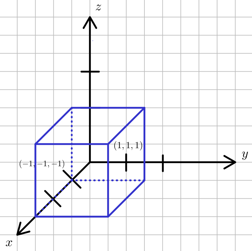 Plainly, if the vertex coordinates are inside this cube, they will be drawn, and if they are outside, they will not. It is worth noting
that this is an arbitary design decision of OpenGL/WebGL, but the viewing region has to determined somehow, and this is a sensible way to do it.
Because our computer monitors are 2-dimensional and not 3-dimensional cubes, the next step WebGL takes is to discard the z-coordinate, effectively
projecting everything inside the cube to the xy-plane. However, it is is important to note that the z-coordinate can still be used by the framework to
determine the order in which objects are drawn. As a final step, WebGL projects the xy coordinates inside the cubes to the actual dimensions
of the WebGL canvas.
Plainly, if the vertex coordinates are inside this cube, they will be drawn, and if they are outside, they will not. It is worth noting
that this is an arbitary design decision of OpenGL/WebGL, but the viewing region has to determined somehow, and this is a sensible way to do it.
Because our computer monitors are 2-dimensional and not 3-dimensional cubes, the next step WebGL takes is to discard the z-coordinate, effectively
projecting everything inside the cube to the xy-plane. However, it is is important to note that the z-coordinate can still be used by the framework to
determine the order in which objects are drawn. As a final step, WebGL projects the xy coordinates inside the cubes to the actual dimensions
of the WebGL canvas.
This spells out our objective quite clearly: the vertices of our 3d scene or object we would like to display should be transformed to coordinates lying inside the cube. Everything else should be mapped somewhere else. Let's look at the following, very simple WebGL scene to illustrate this fact.
Transformation:
=
In the above, a single triangle with the depicted original coordinates is drawn. We then allow each coordinate to be shifted by a constant amount, for example \(x_h = x + \Delta x\). By specifying different values for the constants \(\Delta x, \Delta y, \Delta z\), it is possible to push the transformed vertex coordinates out of the cube, which will result them in not being drawn in our scene.
The way we apply this vertex transformation is by multiplying the depicted
4x4 matrix with the vector representing the vertex with the constant 1 appended
at the last entry. The final transformed coordinates are determined as
\(x' = \dfrac{x_h}{h}\) and analogously for \(y\) and \(z\). Note that both \(x_h\) and \(h\) can be seen as linear functions, with the coefficients represented by
the respective matrix entries: for example \(x_h = ax + by + cz + d\). In the example above,
we set the matrix entries such that \(x_h = x + \Delta x\) and \(h=1\).
This calculus, called homogeneous coordinates, happens to be flexible
enough to represent the usual viewing transformations required for 3d graphics, which is why
it is ubiquitous in the field.
Armed with this information, applying various forms of 3-dimensional projection amounts to doing some simple trigonometry, as we'll discuss in the next section.
Oblique projection of vertices.
Oblique projection refers to one possible way of representing a 3-dimensional object on a 2-dimensional screen. In this form of projection, we want to project an arbitary xyz coordinate onto an xy plane characterized by some fixed z-coordinate \(z_{vp}\) which we specify. The way we carry out this projection is by projecting each coordinate along parallel lines. This line is commonly determined by two angles \(\alpha\) and \(\phi\). The angle \(\alpha\) specifies the intersection angle of the line with the xy-plane. The angle \(\phi\) specifies the angle between the line \(L\) between the points \((x,y,z_{vp})\) and \((x_{vp},y_{vp},z_{vp})\) and the x-axis on the viewing plane. The following sketch summarizes the situation: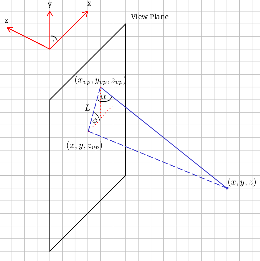
Now, we would like to know the projected coordinates \(x_{vp}, y_{vp}\). From the sketch, we can see that $$ x_{vp} = x + \cos\phi\ L, $$$$ y_{vp} = y + \sin\phi\ L. $$ and that $$ L = (z_{vp}-z) \cot \alpha. $$ We see that \(x_{vp}\) and \(y_{vp}\) are linear functions, and as such we can represent the projection using the following
4x4 matrix and homogenous coordinates.